Chess AI

This work is licensed under a Creative Commons Attribution-ShareAlike 2.0 Generic License.
This is a static version of a Jupyter Notebook, to run the code and experiment it by yourself, click here: ![]()
I admit it. I've also seen Netflix's fascinating hit show: The Queen's Gambit and now I've been playing on chess.com almost every day. With my computer science background I was curious on how can we create a Chess AI, that is, an Artificial Intelligence algorithm that plays the game against a human player. In this article we will see how to create such an algorithm from scratch.

1.- Chess
I suppose you already know chess is a very popular two-player strategy game that originated sometime before the 7th century which is played on a chessboard, a checkered board with 64 squares arranged in an 8×8 grid.
If you are not a chess expert, you probably didn't know that chessboard squares and pieces are given names. The chessboard is split into rows named ranks (1,2, ..., 8) and columns named files (A,B,...,H) so each one of the 64 squares gets a unique name. Pieces are also given a short one letter name so it is easier to name them.

Just like musicians are able to listen the music inside their head from the notes in a music sheet, chess experts are able to play games just by reading symbols:
This may look very complicated, but is just a set of text-like representation of the moves in the game. This notation called Standard Algebraic Notation (SAN), represents a move by the piece's uppercase letter, plus the coordinate of the destination square. However there is an exception to the rule, for pawn moves, the piece letter is omitted and only the destination square is given.
There are some other special symbols like xwhich are placed before the destination square in case of a capture, +indicating check, # indicating checkmate and O-O-O or O-O representing special moves like castling.
Let's see what the first four moves of the previous example would look like:
Now that we have all the knowledge required, let's go!
2.- Minimax AI
How do we create an AI? The very first thing we need to think about is what we want to achieve and then we can go on and think how we can do so. Intuitively we want to win the game, but how can we express that? Well, we know for sure that some pieces are more powerful than others, that checkmating the king is what makes you win the game, but how do you express strategy?, what if sacrificing a piece can actually make us win the game? Well, this is very complicated...
But for a moment let's suppose we can give to every player a score that sums up the number of pieces in the board and the position in the board (for instance, having a rook blocked is worse than having it attacking a piece, and having a pawn is better than not having one).
Let's now simplify what means to win by saying that what we want to achieve is to have, in the near future, a better score than the one of our opponent. Note that by not forcing it to maximise the score at each move, we are allowing sacrifices to be made and leaving room for strategy.
What we know is that computers are very good at performing computations, what if we played out all the possible moves with their help and then choose the one which guarantees us the best score in the near future?
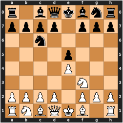
This intuitive idea is encoded by the Minimax algorithm. Each board state is represented by a node with the color of who's turn it is to move. Then from each move, we build out a tree of all the possible moves that can be done from that move on.
Since both players get a score, let's supose that the white player has a positive (+) score and the black player has a negative score (-) so we can easily compare who has an advantage in the game. If at a state we have a negative value, it means black has an edge, while if the value is positive, white has an edge.
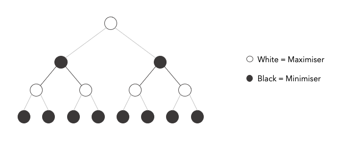
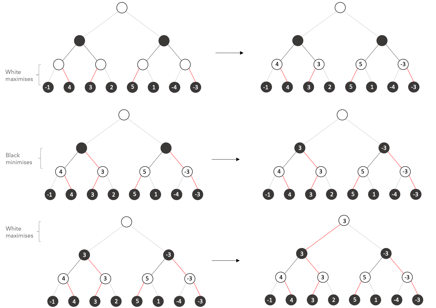
The minimax is an algorithm that simply explores states $n$ moves ahead and selects the action that is guaranteed to give an edge to the player assuming that the other opponent plays optimally. The algorithm is called this way because at each move the black player will aim to minimse the score, while the white player will aim to maximise it, hence minimax.
We just evaluate the states $n$ moves ahead and then assign to each parent node the min/max value according to who is to play.
Here we can see the tree that would be built with a game that for each state has only two valid moves (since each node has only two children). Chess is much more complicated, it is approximated that the average branching factor, that is the average number of possible moves at each state is somewhere about $b=35$. This example shows only tree of depth $d=3$ meaning that the algorithm is looking only at the possible outcomes in the next three moves.
It is easy to see that the number of states we need to consider grows exponentially with the number of moves to consider, that is, we need to analyse approximately: $$ n = b^d \text{ states }$$
What is amazing is that it is estimated that chess Grandmasters can think approximately 14-20 moves ahead! That would be equivalent of considering 4,139,545,122,369,384,765,625 possible states!
However we can build a pretty good chess AI looking only 6 moves ahead, which would consider approximately 1.83 billion states. Such an algorithm is able to achieve approximately an Elo rating of 1966 [1]. But only on Chess.com there would be around 150 people who could beat the algorithm (moreover it is estimated that Beth Harmon reached 2200 ELO). Yikes!
Ok, but how do we assign a score to a board state? For now we will use some heuristics, piece advantage and board position. We will not look to other heuristics such as pawn structures or stategy, we assume looking into future positions will sove the rest.
Here we can see some examples:

Essentially scores are taken according to the strength of a piece, for instance a rook is slightly better than a bishop since a bishop cannot reach squares which are not of its starting color therefore making half the board inaccessible. The position values are instead based on how many squares can the piece can attack (the more the better) and on the positional advantage (control of the center).
Now let's see how this looks concretely in code:
2.1 Python code
import chess
import chess.svg
import numpy as np
from numba import njit
Static evaluation
def evaluate_board(board):
    """Assigns a score to the board according to several metrics:
        - the value of the piece
        - the position of the piece

    Parameters
    ----------
    board : chess.Board
    """
    total_score = 0

    if board.is_checkmate():
        if board.turn == chess.WHITE:
            return -10000
        else:
            return 10000

    for square in chess.SQUARES:
        piece = board.piece_at(square)
        if piece is not None:
            x = chess.square_file(square) # Letter - column
            y = chess.square_rank(square) # Number - row

            value = piece_value[piece.piece_type] + \
                    position_value[piece.piece_type][piece.color][y][x]

            # invert sign if black
            if piece.color == chess.BLACK: value = - value

            total_score += value

    return total_score


""" ----------------------------------------------------------------------
    Positional and Piece Values
    ----------------------------------------------------------------------"""
piece_value = {
    chess.PAWN  : 10,
    chess.BISHOP: 30,
    chess.KNIGHT: 30,
    chess.ROOK  : 40,
    chess.QUEEN : 90,
    chess.KING  : 1000
    }

black_pawn_eval = np.array([
    [0.0,  0.0,  0.0,  0.0,  0.0,  0.0,  0.0,  0.0],
    [5.0,  5.0,  5.0,  5.0,  5.0,  5.0,  5.0,  5.0],
    [1.0,  1.0,  2.0,  3.0,  3.0,  2.0,  1.0,  1.0],
    [0.5,  0.5,  1.0,  2.5,  2.5,  1.0,  0.5,  0.5],
    [0.0,  0.0,  0.0,  2.0,  2.0,  0.0,  0.0,  0.0],
    [0.5, -0.5, -1.0,  0.0,  0.0, -1.0, -0.5,  0.5],
    [0.5,  1.0, 1.0,  -2.0, -2.0,  1.0,  1.0,  0.5],
    [0.0,  0.0,  0.0,  0.0,  0.0,  0.0,  0.0,  0.0]
])

black_rook_eval = np.array([
    [  0.0,  0.0,  0.0,  0.0,  0.0,  0.0,  0.0,  0.0],
    [  0.5,  1.0,  1.0,  1.0,  1.0,  1.0,  1.0,  0.5],
    [ -0.5,  0.0,  0.0,  0.0,  0.0,  0.0,  0.0, -0.5],
    [ -0.5,  0.0,  0.0,  0.0,  0.0,  0.0,  0.0, -0.5],
    [ -0.5,  0.0,  0.0,  0.0,  0.0,  0.0,  0.0, -0.5],
    [ -0.5,  0.0,  0.0,  0.0,  0.0,  0.0,  0.0, -0.5],
    [ -0.5,  0.0,  0.0,  0.0,  0.0,  0.0,  0.0, -0.5],
    [  0.0,   0.0, 0.0,  0.5,  0.5,  0.0,  0.0,  0.0]
])

black_bishop_eval = np.array([
    [ -2.0, -1.0, -1.0, -1.0, -1.0, -1.0, -1.0, -2.0],
    [ -1.0,  0.0,  0.0,  0.0,  0.0,  0.0,  0.0, -1.0],
    [ -1.0,  0.0,  0.5,  1.0,  1.0,  0.5,  0.0, -1.0],
    [ -1.0,  0.5,  0.5,  1.0,  1.0,  0.5,  0.5, -1.0],
    [ -1.0,  0.0,  1.0,  1.0,  1.0,  1.0,  0.0, -1.0],
    [ -1.0,  1.0,  1.0,  1.0,  1.0,  1.0,  1.0, -1.0],
    [ -1.0,  0.5,  0.0,  0.0,  0.0,  0.0,  0.5, -1.0],
    [ -2.0, -1.0, -1.0, -1.0, -1.0, -1.0, -1.0, -2.0]
])

knight_eval = np.array([
    [-5.0, -4.0, -3.0, -3.0, -3.0, -3.0, -4.0, -5.0],
    [-4.0, -2.0,  0.0,  0.0,  0.0,  0.0, -2.0, -4.0],
    [-3.0,  0.0,  1.0,  1.5,  1.5,  1.0,  0.0, -3.0],
    [-3.0,  0.5,  1.5,  2.0,  2.0,  1.5,  0.5, -3.0],
    [-3.0,  0.0,  1.5,  2.0,  2.0,  1.5,  0.0, -3.0],
    [-3.0,  0.5,  1.0,  1.5,  1.5,  1.0,  0.5, -3.0],
    [-4.0, -2.0,  0.0,  0.5,  0.5,  0.0, -2.0, -4.0],
    [-5.0, -4.0, -3.0, -3.0, -3.0, -3.0, -4.0, -5.0]
])

black_king_eval = np.array([
    [ -3.0, -4.0, -4.0, -5.0, -5.0, -4.0, -4.0, -3.0],
    [ -3.0, -4.0, -4.0, -5.0, -5.0, -4.0, -4.0, -3.0],
    [ -3.0, -4.0, -4.0, -5.0, -5.0, -4.0, -4.0, -3.0],
    [ -3.0, -4.0, -4.0, -5.0, -5.0, -4.0, -4.0, -3.0],
    [ -2.0, -3.0, -3.0, -4.0, -4.0, -3.0, -3.0, -2.0],
    [ -1.0, -2.0, -2.0, -2.0, -2.0, -2.0, -2.0, -1.0],
    [  2.0,  2.0,  0.0,  0.0,  0.0,  0.0,  2.0,  2.0 ],
    [  2.0,  3.0,  1.0,  0.0,  0.0,  1.0,  3.0,  2.0 ]
])

queen_eval = np.array([
    [ -2.0, -1.0, -1.0, -0.5, -0.5, -1.0, -1.0, -2.0],
    [ -1.0,  0.0,  0.0,  0.0,  0.0,  0.0,  0.0, -1.0],
    [ -1.0,  0.0,  0.5,  0.5,  0.5,  0.5,  0.0, -1.0],
    [ -0.5,  0.0,  0.5,  0.5,  0.5,  0.5,  0.0, -0.5],
    [  0.0,  0.0,  0.5,  0.5,  0.5,  0.5,  0.0, -0.5],
    [ -1.0,  0.5,  0.5,  0.5,  0.5,  0.5,  0.0, -1.0],
    [ -1.0,  0.0,  0.5,  0.0,  0.0,  0.0,  0.0, -1.0],
    [ -2.0, -1.0, -1.0, -0.5, -0.5, -1.0, -1.0, -2.0]
])

white_pawn_eval = np.flipud(np.fliplr(black_pawn_eval))
white_bishop_eval = np.flipud(np.fliplr(black_bishop_eval))
white_rook_eval = np.flipud(np.fliplr(black_rook_eval))
white_king_eval = np.flipud(np.fliplr(black_king_eval))

position_value = {
    chess.PAWN   : {chess.WHITE: white_pawn_eval, chess.BLACK: black_pawn_eval},
    chess.BISHOP : {chess.WHITE: white_bishop_eval, chess.BLACK: black_pawn_eval},
    chess.KNIGHT : {chess.WHITE: knight_eval, chess.BLACK: knight_eval},            # same for both
    chess.ROOK   : {chess.WHITE: white_rook_eval, chess.BLACK: black_pawn_eval},
    chess.QUEEN  : {chess.WHITE: queen_eval, chess.BLACK: queen_eval},              # same for both
    chess.KING   : {chess.WHITE: white_king_eval, chess.BLACK: black_pawn_eval}
}
Minimax Algorithm
def minimax(board, depth, to_move=None):
    """Minimax Tree evaluation

    Parameters
    ----------
    board : chess.Board
        a chess board with a particular setup (pieces->squares)
    depth : int
        how many moves ahead we want to think
    to_move : chess.Player, optional
        the player whose turn it is to make a move, by default None
    """

    if depth == 0 or board.is_game_over():
        # static evaluation -> end of recursion
        return board.peek(), evaluate_board(board)

    if board.turn == chess.WHITE : # maximise

        max_val = -np.infty
        best_move = None

        # we should explore the tree
        for move in board.legal_moves:
            # simulate the move
            board.push(move)
            # evaluate it
            _, value = minimax(board, depth -1, to_move=chess.BLACK)
            # if best move seen, update it
            if value > max_val:
                best_move = move
                max_val = value
            # take it back
            board.pop()

        return best_move, max_val

    else : # black -> minimise

        min_val = np.infty
        best_move = None

        # we should explore the tree
        for move in board.legal_moves:
            # simulate the move
            board.push(move)
            # evaluate it
            _, value = minimax(board, depth -1, to_move=chess.WHITE)
            # if best move seen, update it
            if value < min_val:
                best_move = move
                min_val = value
            # take it back
            board.pop()

        return best_move, min_val
Let's see it in action!
def play_game(AIcolor=chess.WHITE, depth=3, init_fen=None):

    #start a game with the default setup
    if init_fen is None: init_fen = 'rnbqkbnr/pppppppp/8/8/8/8/PPPPPPPP/RNBQKBNR w KQkq - 0 1'
    board = chess.Board(fen=init_fen)
    chess.svg.board(board, size=250)
    states = []

    if AIcolor == chess.BLACK:
        print('Enter the opponent\'s move')
        opponent_move = input()
        board.push(chess.Move.from_uci(str(opponent_move)))
        states.append(board.fen())

    while not board.is_game_over():
        # AI_move
        best_move, val = minimax(board, depth=depth, to_move=AIcolor)
        print(f'You should play: {best_move}')
        board.push(best_move)
        states.append(board.fen())

        # Opponent move
        print('Enter the opponent\'s move')
        opponent_move = input()
        board.push(chess.Move.from_uci(str(opponent_move)))
        states.append(board.fen())

    return states
Let's suppose that we want to cheat while playing chess. We will enter all our opponent's move and the AI will choose the best move to take having considered all all posible states 3 moves ahead. (Be prepared to wait for long when setting the depth more than three!)
#states = play_game(AIcolor=chess.WHITE, depth=3)
Now let's visualize the game in a GIF!
from PIL import Image
from cairosvg import svg2png
import io
import chess.pgn

def make_gif(game_states, file_name='chess_game.gif'):
    frames = []
    for state in game_states:
        img = svg2png(bytestring=str(chess.svg.board(chess.Board(fen=state), size=250)._repr_svg_()))
        frames.append(Image.open(io.BytesIO(img)))
    frames[0].save(file_name, save_all=True, append_images=frames, duration=100, loop=0, optimize=False)

def pgn_gif(file, gif_name='pgn_game'):
    states = []
    game = chess.pgn.read_game(open(file))
    board = game.board()

    for move in game.mainline_moves():
        board.push(move)
        states.append(board.fen())

    make_gif(states, file_name=f'chess_imgs/{gif_name}.gif')
# make_gif(states, file_name='chess_game.gif')
# you can simulate the game on lichess.com and then download the PGN and load it here
# below to see a GIF of your game
# pgn_gif('lichess.pgn')

2.- Alpha-Beta Pruning + Minimax
Even if our algorithm works, it would be painfully slow... No one wants to wait 30 min for the AI to make a move, so we normally limit it to explore future states at a reasonable depth. Note that our algorithm is pretty weak as we only consider a depth of 3. But we previously mentioned that grandmasters are able to play as if they saw 14-20 levels of depth! Our algorithm takes a lot of time for a few levels, how can they compute all those levels? Well, they are so experienced that they already know that most of the states will never be reached, so they can efficiently explore the future states that actually matter, not all of them. What if there was an optimisation that would allow us to descend deeper into the tree without necessarily taking more computation time, similar to what grandmasters do? Such optimisation exists and is called alpha-beta pruning. It is called this way because we use two parameters: $\alpha$ and $\beta$, to prune the tree, that is to cut off some branches and avoid computing useless future states.
This optimisation is based on the simple idea: "the opponent plays optimally, no sense to compute branches that will result in a bigger advantage for me, as he will play so that my advantage is minimised"
Let's see the following tree. Normally we would have to explore all the states at the final depth, that is we would need to perform an evaluation of the current situation (who has an advantage) at at least 8 states.
![]()
Instead of building the tree by depth level like we did before, let's try to build the tree by subtrees like shown in the animation.
Now let's repeat the process taking into account the fact that the opponent plays optimally:
Let's see the final state:
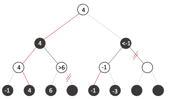
It is important to remark the fact that we avoided the computation of 3/8 states because their value is irrelevant, you can try any number you want on the states and the result would never change.
Let's look closely how it works. When we arrive at the third state, At this point when we explore
But how do we formalise such mechanism. We simply keep two extra variables: alpha and beta:
- alpha $\alpha$: represents the highest value encountered. Set by maximiser player (white). By default $-\infty$.
- beta $\beta$: represents the lowest value encountered. Set by minimiser player (black). By default $+\infty$.
$\beta \leq \alpha$ -> prune unvisited subtrees
from tqdm.notebook import tqdm

def pruning_minimax(board, depth, alpha=None, beta=None, to_move=None):
    """Minimax Tree evaluation improved by not considering positions
    that can't affect the outcome.

    Parameters
    ----------
    board : chess.Board
        a chess board with a particular setup (pieces->squares)
    depth : int
        how many moves ahead we want to think
    alpha : int, optional
        highest value in the subtree, by default -np.infty
    beta : int, optional
        lowest value in the subtree, by default np.infty
    to_move : chess.Player, optional
        the player whose turn it is to make a move, by default None
    """
    if alpha is None : alpha = -np.infty
    if beta is None : beta = np.infty

    if depth == 0 or board.is_game_over():
        # static eval - end of recursion
        return board.peek(), evaluate_board(board)


    if board.turn == chess.WHITE : # maximise

        max_val = -np.infty
        best_move = None

        # we should explore each tree branch
        for move in board.legal_moves:

            # simulate the move (explore the branch)
            board.push(move)

            # evaluate it
            _, value = pruning_minimax(board, depth -1, alpha, beta, to_move=chess.BLACK)

            # if best move seen, update it
            if value > max_val:
                best_move = move
                max_val = value

            # take it back (return to parent)
            board.pop()

            alpha = max(alpha, value)
            # no sense checking other options as the player is not
            # likely to choose this branch under the hypothesis
            # he performs the best move, otherwise if he does he
            # will end in a situation worse for him
            if beta <= alpha: break

        return best_move, max_val


    else : # black -> minimise

        min_val = np.infty
        best_move = None

        # we should explore the tree
        for move in board.legal_moves:

            # simulate the move (explore the branch)
            board.push(move)

            # evaluate it
            _, value = pruning_minimax(board, depth -1, alpha, beta, to_move=chess.WHITE)

            # if best move seen, update it
            if value < min_val:
                best_move = move
                min_val = value

            # take it back (return to parent)
            board.pop()

            beta = min(beta, value)
            # no sense checking other options as the player is not
            # likely to choose this branch under the hypothesis
            # he performs the best move, otherwise if he does he
            # will end in a situation worse for him
            if beta <= alpha: break

        return best_move, min_val
Let's see it in action!
def play_game(AIcolor=chess.WHITE, depth=3, init_fen=None):

    #start a game with the default setup
    if init_fen is None: init_fen = 'rnbqkbnr/pppppppp/8/8/8/8/PPPPPPPP/RNBQKBNR w KQkq - 0 1'
    board = chess.Board(fen=init_fen)
    chess.svg.board(board, size=250)
    states = []

    if AIcolor == chess.BLACK:
        print('Enter the opponent\'s move')
        opponent_move = input()
        board.push(chess.Move.from_uci(str(opponent_move)))
        states.append(board.fen())

    while not board.is_game_over():
        # AI_move
        best_move, val = pruning_minimax(board, depth=depth, to_move=AIcolor)
        print(f'You should play: {best_move} Approx Value: {val}')
        board.push(best_move)
        states.append(board.fen())

        if board.is_game_over(): break

        # Opponent move
        print('Enter the opponent\'s move')
        opponent_move = input()
        board.push(chess.Move.from_uci(str(opponent_move)))
        states.append(board.fen())

    print(f'Result White {board.result()} Black')
    return states
Take a look at this game of the AI just built against Aaron BOT AI (~ELO 700) at chess.com. Feel free to reproduce the whole game uncommenting the line below. The AI we just built won with an accuracy of 94.20% w.r.t. to a top class AI! Not bad!

# states = play_game(AIcolor=chess.WHITE, depth=5)
Did you notice the speed increase with respect to the previous version? In the ideal case, we can double the depth at the same computational complexity! And that is a lot! That difference is like the one between an amateur and a world master! However, alpha-beta pruning is highly dependent on the order in which each node is examined.
3.- Further Improvements
3.1- Zobrist Hashing
What happens with the current algorithm is that we might visit the same state multiple times. For example we can perform a couple of moves where the final state is the same, we must compute the score for the same state, multiple times. An idea could be to save the score for the state and then when we encounter that state again, we just used the value computed before. The question that naturally arises is: how can we save such values? To do so, we must implement a process to for creating a unique identifier out of the board so we can then retrieve the value when encountered again. But we need to do so efficiently, meaning that this process should be fast enough to justify the fact that to load the value is better than to recompute it again.
The solution to this problem is to use a transposition table, a special kind of hash table that is indexed by board position. To generate an index out of the board position we use Zobrist hashing, a hash function invented by Albert Lindsey Zobrist which uses randmly generated bitstrings for every possible combination of a piece and position. Meaning that each of the 64 squares of the board will have associated 13 bitstrings, 12 for each the pieces and one associated to the fact of being empty.
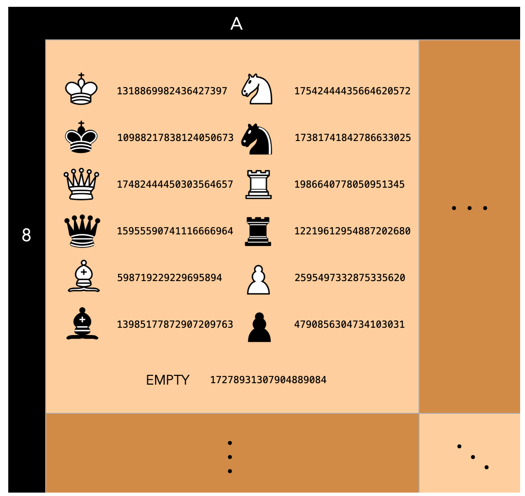
Although it is possible that two numbers out of the 13 x 64 = 832 are the same, the probability should be so low that it is almost impossible.
import random
# init hash table / dict
transposition_table = {}
# Pieces encoding color and piece type:
PIECES = [chess.Piece.from_symbol('P'), chess.Piece.from_symbol('B'),
          chess.Piece.from_symbol('N'), chess.Piece.from_symbol('R'),
          chess.Piece.from_symbol('Q'), chess.Piece.from_symbol('K'),
          chess.Piece.from_symbol('p'), chess.Piece.from_symbol('b'),
          chess.Piece.from_symbol('n'), chess.Piece.from_symbol('r'),
          chess.Piece.from_symbol('q'), chess.Piece.from_symbol('k'),
          'EMPTY']

#initialise
for square in chess.SQUARES: transposition_table[square] = {}
# generate a random number for every square/piece combination
for square in chess.SQUARES:
    for piece in PIECES:
        transposition_table[square][piece] = random.getrandbits(64)
def zobrist_hash(board):
    h = 0

    for square in chess.SQUARES:
        piece = board.piece_at(square)
        if piece is not None:
            h ^= transposition_table[square][piece]
        else:
            h ^= transposition_table[square]['EMPTY']

    return h
Zobrist hash has some really nice properties, in fact, it is possible to efficiently recompute the hash from one position to another by simply XORing IN or OUT the changes in the board.
This is due to the XOR function: $$A\oplus B = {\displaystyle (A\cdot {\overline {B}})+({\overline {A}}\cdot B)\equiv (A+B)\cdot ({\overline {A}}+{\overline {B}})}$$
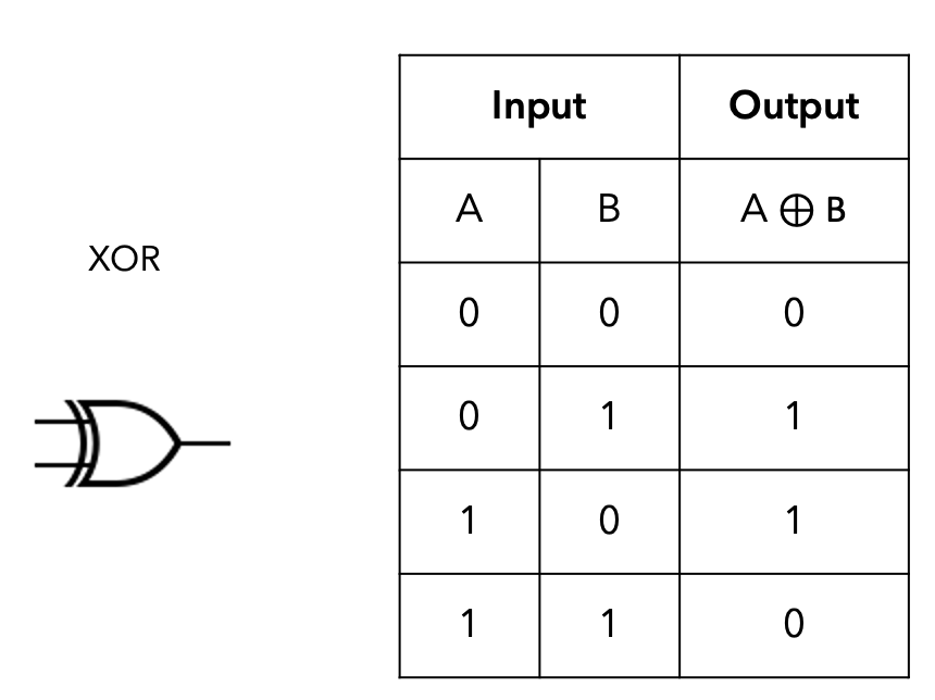
In fact, the XOR function is "reversible" ($ A\oplus B \oplus B = A $):
$$ \begin{align} C = A\oplus B \quad \Rightarrow \quad C \oplus B &= (C\cdot {\overline {B}})+({\overline {C}}\cdot B)\\ &= ([(A\cdot {\overline {B}})+({\overline {A}}\cdot B)]\cdot {\overline {B}})+({\overline {[(A\cdot {\overline {B}})+({\overline {A}}\cdot B)]}}\cdot B)\\ &= [(A\cdot {\overline {B}})\cdot {\overline {B}}+({\overline {A}}\cdot B)\cdot {\overline {B}}]+[{\overline {(A\cdot {\overline {B}})}+\overline{({\overline {A}}\cdot B)}}]\cdot B\\ &= A\cdot {\overline {B}}+[(\overline {A}+ \overline {\overline {B}}) + (\overline{\overline {A}}+\overline{B})]\cdot B\\ &= A\cdot {\overline {B}}+[\overline {A}+ B + A+ \overline{B}]\cdot B\\ &= A\cdot {\overline {B}}+[1]\cdot B\\ &= A\cdot ({\overline {B}} + B)\\ &= A \end{align} $$Moreover the XOR operation is an operation that can be efficiently performed by the computer, meaning that with a proper implementation this operation can be performed efficiently.
Disclaimer: in the example below we might not see an advantage in terms of performance when computing the hash from scratch and when recomputing the hash based on the previous hash, this is due to the not so performant nature of Python which trades-off performance for flexibility and readability.
from collections import namedtuple
def recompute_zobrist_hash(board, prev_hash, move):
    """Efficiently recomputes the hash of the new state.
    Assumes move is yet to be pushed.

    Parameters
    ----------
    prev_hash : [type]
        the zobrist hash at the previous move
    move : chess.Move
        the move taken at the last turn which lead to the new board state
        in case of castling this is a set of two moves
    """

    new_hash = prev_hash
    Move = namedtuple('Move', ['from_square', 'to_square'])

    # create pseudo moves for castling
    if move == chess.Move.from_uci('e8a8') : # black queen-side castling 0-0-0
        moves = [Move(chess.E8, chess.C8), Move(chess.A8, chess.D8)]
    elif move == chess.Move.from_uci('e8h8') : # black king side castling 0-0
        moves = [Move(chess.E8, chess.G8), Move(chess.H8, chess.F8)]
    elif move == chess.Move.from_uci('e1a1') : # white queen side castling 0-0-0
        moves = [Move(chess.E8, chess.G8), Move(chess.H8, chess.F8)]
    elif move == chess.Move.from_uci('e1h1') : # white king side castling 0-0
        moves = [Move(chess.E8, chess.G8), Move(chess.H8, chess.F8)]
    else:
        moves = [move]
    # doesn't handle promotion or en-passant, but you get the idea..


    for move in moves :

        piece = board.piece_at(move.from_square)

        # XOR out piece from old position
        new_hash ^= transposition_table[move.from_square][piece]

        # XOR in empty at old position
        new_hash ^= transposition_table[move.from_square]['EMPTY']

        # XOR in piece at new position
        new_hash ^= transposition_table[move.to_square][piece]

        captured_piece = board.piece_at(move.to_square)
        if captured_piece is not None:
            # XOR out position of captured piece
            new_hash ^= transposition_table[move.to_square][captured_piece]
        else:
            # XOR out empty at new position
            new_hash ^= transposition_table[move.to_square]['EMPTY']

        return new_hash
Example:
b = chess.Board()
prev_hash = zobrist_hash(b)
prev_hash
recompute_zobrist_hash(b, prev_hash, chess.Move.from_uci('e2e4'))
b.push(chess.Move.from_uci('e2e4'))
zobrist_hash(b)
Note that the hashes yield the same value whether it is recomputed from scratch or by XORing IN or OUT the changes.
3.2- Iterative Deepening
Iterative deepening (IDS) is an algorithm used to visit a tree. It is an alternative to the commonly used Depth-first Search (DFS) or Breath-first Search (BFS). This algorithm acts like a depth-bounded DFS with increasing depth parameter like we can observe in the animation.
Since iterative deepening visits states multiple times, it may seem wasteful, but it turns out to be not so costly, since in a tree most of the nodes are in the bottom level, so it does not matter much if the upper levels are visited multiple times, it matters even less if we use a transposition table to save the score of the visited state.
This kind of algorithm provides two main advantages:
- we can use searches at smaller depth to improve alpha-beta heuristics (alpha–beta pruning is most efficient if it searches the best moves first).
- we can return the best move at any time. By repeating the process, each time with one level in depth more, we are able to return the current best move at any time. This is particularly useful if we have time constraints. For example, we can descend the tree for 30 seconds, then we will return the answer, in the openings probably there are fewer moves than in the endgame, thus in the openings we might be able to descend deeper into the tree.
Conclusion!
Et Voilà! You now understand the main concepts behind IBM's Deep Blue, the computer who managed to beat Garry Kasparov in 1997. With the only differences being the fact that Deep Blue used 512 VLSI chips in parallel to execute the alpha-beta search algorithm thus mitigating the problems concerning the computational tractability, it used a kind of book for openings and endings and used uneven tree development exploring some branches deeper (for instance when a piece was captured or when there was a check). But you already know the core concepts!
Today the Artificial Intelligence has advanced a lot and today, Deep Blue's technique is considered quite old. In the last decade there has been a surge of better algorithms which use Reinforcement Learning and avoid the computation of million of states.
In the image below we can see the evolution of several chess AI algorithms...
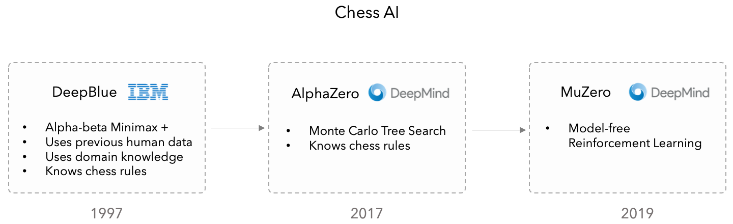
but today Chess has lost its spark mainly because computers are better than us... The attention has shifted towards the game of Go which is much more complicated. The number of legal board positions in Go has been calculated to be approximately $2.1 \times 10^{170}$ which is greater than the number of atoms in the observable universe ($10^{80}$)! So in order to beat humans we needed new, more intelligent strategies.